Fine-tunning Stable Diffusion Models using Textual Inversion

Textual Inversion

Textual Inversion(TI) is another way to fine tune the pretrained model. Unlike LoRA, TI is a technique to add new embedding space based on the trained data. Simply put, TI is a text embedding that matches the target image the best, such as its style, object, or face. The key is to find the new embedding that does not exist in the current text encoder.

How does TI works

A latent diffusion model can use images as guidance during training. For training a TI model, we will follow the same pipeline from the previous article, using a minimal set of three to five images, though larger datasets often yield better results.

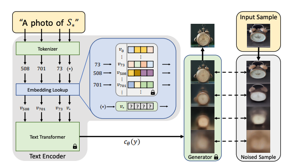
The goal of training is to find a new embedding represented by $v_$. We use $S_$ as the token string placeholder to represent the new concepts we wish to learn. We aim to find a single word embedding, such that sentences of the form “A photo of S*” will lead to the reconstruction of images from our small training set. This embedding is found through an optimization process shown in the above figure, which we refer to as "Textual Inversion".

For example, let’s say we have 5-7 images of a new object, like a custom teddy bear. We want the model to learn what this plush toy looks like. Instead of describing the object in words (e.g., “a teddy bear”), we use S* in the prompt:

• “A photo of S* in a forest”
• “S* sitting on a table”
• “A close-up of S* with soft fur”

Here, S* starts as a meaningless embedding, but during training, it gradually learns the visual characteristics of the teddy bear. After training S* now represents the teddy bear in latent space. You can use it in new prompts:

• “S* in a futuristic city”
• “A cartoon drawing of S*”
• “S* as a superhero”

Now, let talk about the v*. First, recall that the loss function we use to train a latent diffusion model:

The right-hand side is an optimization objective, meaning we are minimizing a loss function, where

• $\epsilon$: The actual noise that was added to the latent representation.
• $\epsilon_{\theta}(z_t, t, c_{\theta}(y))$: The model’s predicted noise at time $t$.

The loss term measures the difference between two noise:

So, the right-hand side ensures the model learns to predict the noise accurately, which is key in a diffusion model.

TI reuses the same training scheme as the original LDM model, while keeping both $c_{\theta}$ and $e_{\theta}$ fixed. Our optimization objective is to find the optimal $v_{*}$ that minimizes the loss above.

Since we are learning a new embedding $𝑣_{∗}$, we do not have a predefined text embedding, that’s why the loss function for TI looks like this:

The equation above does not say the embedding equals the loss. Instead, we say v∗ is the embedding that, when used, results in the smallest possible noise prediction loss.

What This Means is that

• Instead of using a fixed text embedding, we introduce $v$, which is a trainable vector.
• We find the best embedding $v_{*}$ that minimizes the LDM loss by optimizing $v$ over multiple training images.
• The argmin notation means we are searching for the best $v$ that minimizes the noise prediction error.

Once the new corresponding embedding vector is found, the training is done. The output of the training is usually a vector with 768 numbers in the format of pt or bin file. The files are typically just a few kilobytes in size. This makes TI a highly efficient method for incorporating new elements or styles into the image.

For example, the code below loads a TI model(a bin file) from the Hugging Face concepts library. The bin structure is just a key-value pair:

import torch
loaded_leared_embeds = torch.load('/Volumes/ai-1t/ti/midjourney_style.bin', map_location='cpu')
keys = list(loaded_leared_embeds.keys())
for key in keys:
    print(key, ": ", loaded_leared_embeds[key].shape) # <midjourney-style> :  torch.Size([768])

TI in practice

To use TI models, we could just leverage the load_textual_inversion method from the StableDiffusionPipeline

pipe.load_textual_inversion(
    "sd-concepts-library/midjourney-style",
    token = "midjourney-style",
)

This method does two things:

• Registers a New Learnable Token
  • midjourney-style is now a special token in the text encoder.
  • Instead of being processed as a normal word, it is mapped to a learnable embedding vector.
• Replaces midjourney-style in the Text Encoding Step
  • Whenever midjourney-style appears in a prompt, it is replaced with the trained embedding vector (which is equivalent to S* in our previous discussions).
  • The Stable Diffusion model does not process midjourney-style as normal text anymore. It uses the learned latent representation instead.

Now, we can compare the results with and w/o using TI:

Resources

• An Image is Worth One Word: Personalizing Text-to-Image Generation using Textual Inversion
• Using Stable Diffusion with Python